OCV, AOCV, and POCV

• In OCV, a fixed delay factor is applied to the delay of all the cells present in the design. If process variation affects the delay of any cells during fabrication, it will not affect the timing requirements, and the chip will not fail after fabrication.
• Variations in the fabrication process could either increase or decrease the delay of a cell. So, we must set early and late values while setting the derate factor. The STA tool would consider early or late timing derate based on the path and type of analysis.

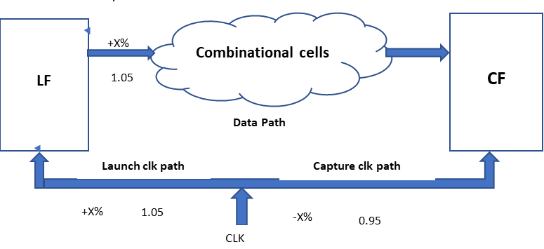
Fig1: Derate Factor on Setup Analysis

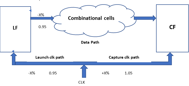
         Fig2: Derate Factor on Hold Analysis

• Figs. 1 and 2 show the derate factor considered by the STA tool during setup and hold analysis for different paths. In reg2reg path timing analysis, there is a launch flop from where data is launched and a capture flop from where data is captured.
• The path from the clock source to the clock pin of the launch flop is called the launch clock path, and the path from the clock source to the clock pin of the capture flop is called the capture clock path.
• In setup analysis, the worst case could be a late data path, a late launch clock path, or an early capture clock path, which could fail the setup timing. So, the STA tool will consider a late timing derate for the data path and launch clock path and an early timing derate for the capture clock path.
• For hold analysis, a fast data path, an early launch clock, and a late capture clock could be the worst scenarios. So, the STA tool will always consider the worst scenario and take the early derate factor for the data path and launch clock path and the late derate factor for the capture clock path.

Issues in OCV:

• The fixed timing rate used for all the cells in the OCV is overly pessimistic.
• In reality, there is a cancellation of the random variation effect. All the cells in a particular path could not be delayed or early.
• There is always a mixed type of effect, and this causes the cancellation of the effect in total.
• The concepts of OCV fixed derate were modelled in the technology node above 90 nm. It was good for such high-tech nodes.
• But in lower-technology nodes and especially high-frequency designs, the timing closure became difficult due to the high pessimism of fixed derate.
• So, for the lower technology node, we need to resolve this issue. And so the concept of Advance On-Chip Variation (AOCV) has evolved, which does not use the fixed derate.

 

Advance On-Chip Variation (AOCV):

• In AOCV, derate is applied to each cell based on the path depth and distance of the cell in the timing path, and it also varies with the cell type and drive strength of the cell. Distance is defined by a bounding box for the net and cell, as shown in Figure 3. 

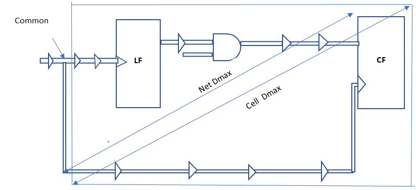
                 Fig3: Bounding box for cell and net distance

Distance: If the distance increases, systematic variation will increase, and to mitigate the variation, we need to use a higher derate value. So along with the distance, the derate value increases.

Path depth: If the distance is fixed and path depth increases, systematic variation would be constant, but random variation would tend to cancel each other. Therefore, as path depth increases, the derate factor decreases.

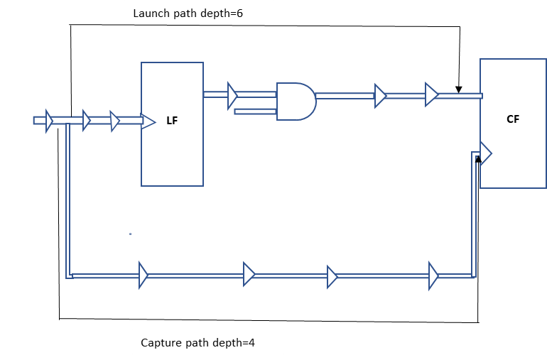
Fig. 4: Path depth in the timing path

Cell type: The derate is based on the cell type, as an AND gate and an OR gate cannot exhibit the same variation. The derate value also varies with the drive strength of the cell; for example, AND2X2 and AND2X6 will have different drive derate values.

AOCV Analysis Mode:

AOCV supports two analysis modes:

1. Clock only
2. Clock and data

In clock-only mode, AOCV derate is applied only on the clock path, so it has reduced effort and a fast runtime. whereas in clock and data modes, AOCV derate is applied on full design. AOCV analysis requires an AOCV derate table for all the cells. Due to reduced timing pessimism in AOCV, it has been observed that huge time violations were fixed when we moved to clock-only AOCV derate mode, and the violations were further reduced when we moved to clock and data.

Setup	2	4	6
10	1.10	1.08	1.04
20	1.15	1.10	1.06
30	1.17	1.13	1.09

Fig5: AOCV 2D derate table example

Prime Time AOCV Flow:

• There are some additional steps added in AOCV derate analysis as compared to OCV fixed derate flow. A flow of the primetime tool for AOCV derate analysis is shown in Fig. 6.
• AOCV analysis supports multiple AOCV derating tables. There are generally two types of tables used: 1D tables and 2D tables. 1D tables contain variation of derate values either with distance or depth, whereas the AOCV 2D derate tables contain derate variation with both distance and depth together.

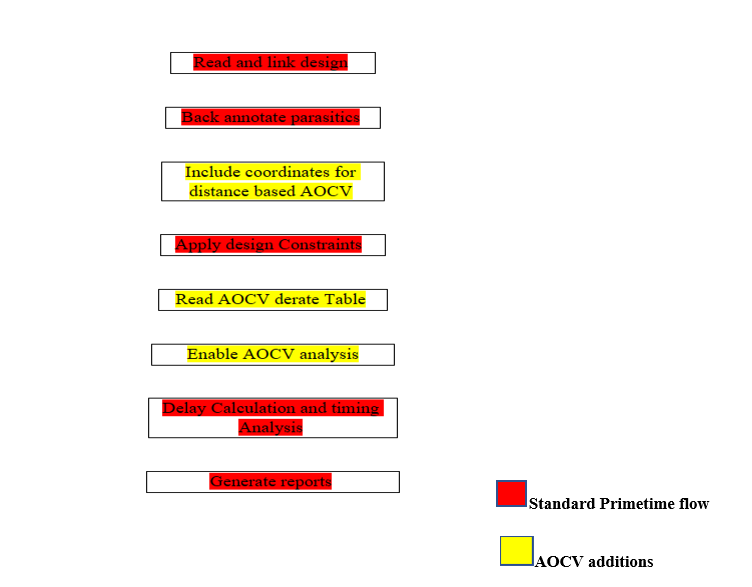
Fig6:PrimeTime AOCV Analysis Flow                                                         

Issues in AOCV:

• AOCV does not perform very well below 40nm technology node and to improve that we need to improve the timing pessimism further.
• Distance and Depth based derate factor used in the AOCV is good for technology nodes above 40nm but for the below node, we need to improve it further.
• To address these issues Parametric On-Chip Variation (POCV) has been developed. POCV is very effective in technology nodes 20nm and below.
• POCV is a more realistic approach than that of OCV and AOCV. This method does not use distance and depth based derate factors.
• It uses delay sigma to model the delay variation of the cell. An advantage of POCV over AOCV is also that it reduces the slack pessimism between Graph-Based Analysis (GBA) and Path Based Analysis (PBA).

Parametric On-chip Variation (POCV):

• POCV advance variation technology provides statistical benefits without the overhead of expansive statistical library characterization.
• In POCV instead of applying the specific derate factor to a cell, cell delay is calculated based on the delay variation (σ) of the cell.
• In POCV it is assumed that the normal delay value of a cell follows the normal distribution curve
• In normal distribution 68% of data falls within the 1σ range, 95% data falls within 2σ and 99.7% data falls within the range of 3σ.  

POCV Analysis:

• POCV uses a nominal delay value (µ) instead of using the min or max value of delay to model the random variations.
• Timing analysis is done using the nominal delay value (µ) and delay variation (σ) in the following way.
  • Tool takes the value of σ from the timing library or an external file containing the POCV coefficient value C.
  • Each arc time is then calculated statistically as the total nominal delay and the variation.
  • The tool then calculates the delay of the path by statistically combining these arc delays and performing the setup and hold timing analysis.
• By default, the tool performs the POCV analysis at 3σ from the mean, but other values can also be specified. The more the value of the standard deviation, it’s more pessimistic in timing.

POCV Delay Calculation:

PrimeTime POCV analysis flow:

A flow of the primeTime tool for POCV derate analysis has shown in figure 8.

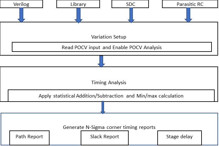
Fig 7: PrimeTime POCV analysis flow

 Comparison between POCV and AOCV:

• A basic comparison between POCV and AOCV has shown below.

AOCV	POCV
Random Variation is modeled through the depth based derate and Systematic Variation is modeled through distance based derate.	Random and Systematic Variations are modeled through a delay variation coefficient which is specific to each cell.
Less accurate correlation between GBA and PBA.	More accurate correlation between GBA and PBA.
Transition Variation and cell check variation are not supported.	Transition Variation and cell check variation supported.

Disclaimer:

The purpose of this blog is to spread knowledge and facilitate open discussions. The content shared is based on our research from diverse sources including the internet, books, and conversations with others. We strive for accuracy; however, we acknowledge the possibility of errors or omissions. We value your input and encourage you to share your comments, questions, and suggestions. We are open to clarifying or correcting any inaccuracies found within the blog. 

Please note that while we appreciate your contributions, we may not be able to implement all suggestions. The blog should not be considered a substitute for professional advice.